
library(tidyverse) # for plotting and data wrangling
library(hmetad) # for confidence modeling
library(tidybayes) # for wrangling posteriors
library(bayestestR) # for significance testing
options(mc.cores = parallel::detectCores()) # fit models in parallelQuantifying metacognitive performance with the hmetad package in R
Installation
In order to complete the tutorial, you will need three things:
A working installation of
R(download here)A working installation of RStudio (or your preferred code editor; download here)
A working installation of the
hmetadpackage (documentation here).hmetaddepends on thebrmspackage, which in turn requires aC++compiler and an installation of the probabilistic programming language Stan. If this is already set up on your computer, you should be able to proceed using theRcommandinstall.packages("hmetad"). If this does not work, please follow the instructions at https://mc-stan.org/install/ to get Stan running on your computer. In particular, on Windows machines, you will need to install Rtools before installinghmetad.
Instructions
The goal of this workshop is to obtain a working knowledge of how metacognition is measured, how it is modeled, and how Bayesian modeling can help to this end. It is not to make you an expert in R programming. So, rather than being asked to write the code on your own, this tutorial provides pre-written code that you can run, adjust, and re-run to get a better understanding of what is going on.
To follow the tutorial, create a blank R script or notebook. As you progress, simply copy each code block into your script and run it (there is a copy button on the right side of each code block). Feel free to fiddle with things until you feel you understand what is going on. When you’re done, not only will you hopefully have a better intuition for Bayesian models of metacognition, but you will also have a lot of template code that you can use in your own projects!
Setup
First, we will need to start a fresh R session and include some necessary packages:
Let’s also load some helper functions to make plots for us:
source("https://github.com/metacoglab/hmetad_workshop/raw/refs/heads/main/tutorial/hmetad_tutorial_utils.R")A descriptive perspective on metacognitive sensitivity
One of the best ways to understand a model is to take some parameter values, simulate some data, and then to see how the simulated data changed as a function of different parameters. First, let’s simulate a large dataset with a default set of parameters (we’ll use this as a reference later on):
d <- sim_metad(N_trials = 10000, dprime = 1.5)
dOutput
As you can see, this function gives us a dataset with one row for each of 1,000 trials, the stimulus that was presented on that trial (0 or 1), the simulated type 1 response (0 or 1), and the simulated confidence level (1, 2, 3, or 4), along with the parameter values used to simulate the data.1
We are often interested in quantifying metacognitive sensitivity: the relationship between confidence ratings and objective performance. To see this directly, we can plot the probability of each confidence rating given a correct or incorrect decision:
plot_confidence(d)Output
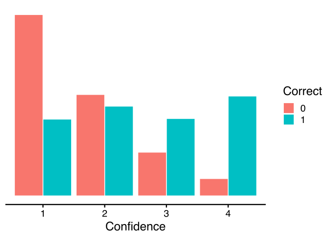
From here it is easy to see that confidence ratings are generally higher for correct responses compared to incorrect responses. This is an indicator of high metacognitive sensitivity: participants are aware of when they are likely to be making a mistake.
Another way to visualize metacognitive performance is to make a type 2 receiver operating characteristic (ROC) curve. This plot shows us, for each possible level of confidence k, the probability of making a confidence rating greater than k for correct and incorrect decisions. That is, we can slide a line between each confidence level, calculate the proportion of correct and incorrect responses to the right of the line, and then plot the proportions against each other:
plot_roc2(d)Output
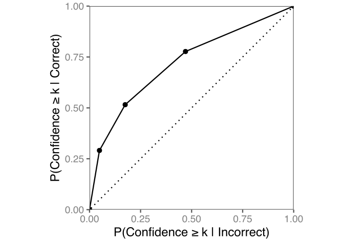
Since confidence ratings are higher for correct decisions than incorrect decisions, this simulated type 2 ROC curve is above the diagonal.
ExerciseExercise: understanding the type 2 ROC
What would the type 2 ROC look like if confidence ratings were the same for correct and incorrect responses?
What would the type 2 ROC look like if confidence ratings perfectly separated correct and incorrect responses?
AnswerSolution
If confidence ratings were equally distributed for correct and incorrect responses, the type 2 ROC would lie on the main diagonal (the dashed line in the plot above). This is because confident responses are equally likely for correct and incorrect responses.
If confidence ratings perfectly separated correct and incorrect responses, the type 2 ROC would make a right angle along the upper left boundary of the plot. For example, imagine that confidence ratings were < 2 for incorrect responses and > 2 for correct responses. If we place a confidence criterion at 2, then, all of the incorrect responses would be to the left of the criterion (indicating a type 2 false alarm rate of 0) and all of the correct responses would be to the right of the criterion (indicating a type 2 hit rate of 1).
How do differences in metacognition manifest?
In order to see what might happen when metacognition is impaired, we can simulate a new dataset with reduced metacognitive efficiency, combining both simulated datasets using bind_rows for convenience (we’ll explain what these parameters mean in more detail later on):
# label the previous dataset as "high" metacognition
d <- d |> mutate(metacognition = "high")
# create a new dataset with "low" metacognition and join them together
d_metacognition <- sim_metad(N_trials = 10000, dprime = 1.5, M = exp(-1)) |>
mutate(metacognition = "low") |>
bind_rows(d)
d_metacognitionOutput
To visualize metacognitive sensitivity, let’s plot confidence directly as a function of accuracy:
plot_confidence(d_metacognition, metacognition)Output
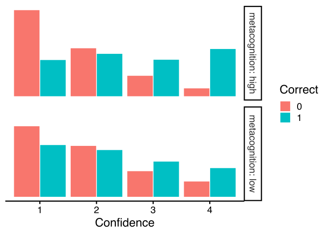
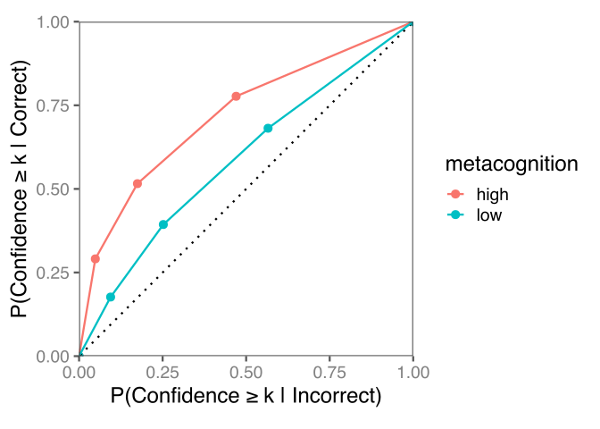
In constrast to the previous case, when metacognitive efficiency is reduced, correct and high confidence responses are less likely, whereas incorrect but high confidence responses are more likely. Intuitively, this also means that the type 2 ROC is closer to the diagonal:
plot_roc2(d_metacognition, metacognition)Output
How does performance change metacognition?
These visualizations are extremely useful in terms of getting an intuition for metacognitive performance, but unfortunately they are not perfect. In particular, these plots are sensitive not only to metacognitive efficiency, but also to task performance (measured by d’) and response bias (measured by c). To get an idea of what this means, let’s simulate another dataset with the same metacognitive efficiency as before but reduced task performance (again, combining both simulated datasets for convenience):
# label the previous dataset as "high" performance
d <- d |> mutate(performance = "high")
# create a new dataset with "low" performance and join them together
d_performance <- sim_metad(N_trials = 10000, dprime = .5) |>
mutate(performance = "low") |>
bind_rows(d)
d_performanceOutput
Again, let’s plot confidence directly as a function of accuracy:
plot_confidence(d_performance, performance)Output
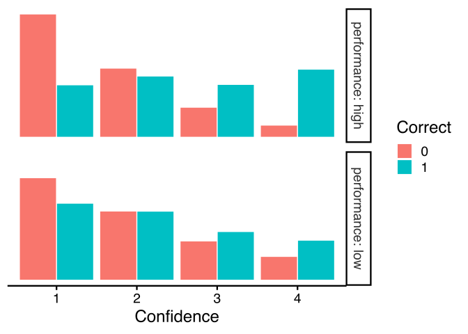
Huh, well that’s strange- just by visually comparing the distributions, the low performance distribution looks very similar to the “low metacognition” distribution from earlier! Again, correct and high confidence responses are less likely, whereas incorrect but high confidence responses are more likely. We see the same pattern for the type 2 ROC:
plot_roc2(d_performance, performance)Output
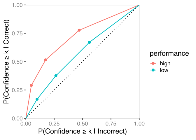
What is going on here? While each of these visualizations provides an absolute measure of metacognition, it turns out that the difficulty of metacognition scales with task difficulty. That is, it is much easier to determine whether your response is correct or not when you have a high accuracy to begin with. This hopefully makes sense in hindsight: if you are very good at a task, even if you have no insight into the accuracy of your individual responses, you can appear to have great metacognition by just rating high confidence most of the time!
In general, there are two kinds of approaches to dealing with this problem:
- Carefully control for task performance using careful psychophysical manipulations
- Explicitly model the relationship between task performance and metacognition to compute a relative measure of metacognition.
In this tutorial we will focus on one version of the latter approach known as the meta-d’ model.
A glimmer of hope
Of course, it sounds great to be able to wave a magical statistical wand to separate cognitive and metacognitive performance from responses and confidence ratings alone. But didn’t all of our data look the same regardless of whether task performance or metacognition was impaired? One might doubt that we can ever make a clean separation between cognitive and metacognitive performance.
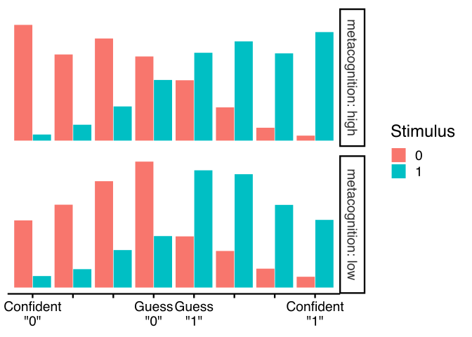
To get an intuition for how this is possible, let’s instead plot the joint distribution of type 1 and type 2 responses. In this plot, the type 1 and type 2 responses are combined into a single joint response, where values on the ends of the scale correspond to different type 1 responses with high confidence, and values in the middle of the scale correspond to guesses:
plot_joint_response(d_metacognition, metacognition)Output
plot_joint_response(d_performance, performance)Output
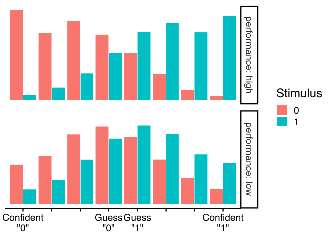
Since these plots show both type 1 responses and confidence ratings, they have a lot more going on. But, comparing the four histograms, it is also clear that there actually is a difference between reduced metacognition and reduced performance! While participants still discriminate strongly between the two stimuli with reduced metacognition, the distributions of responses look very similar for reduced performance.
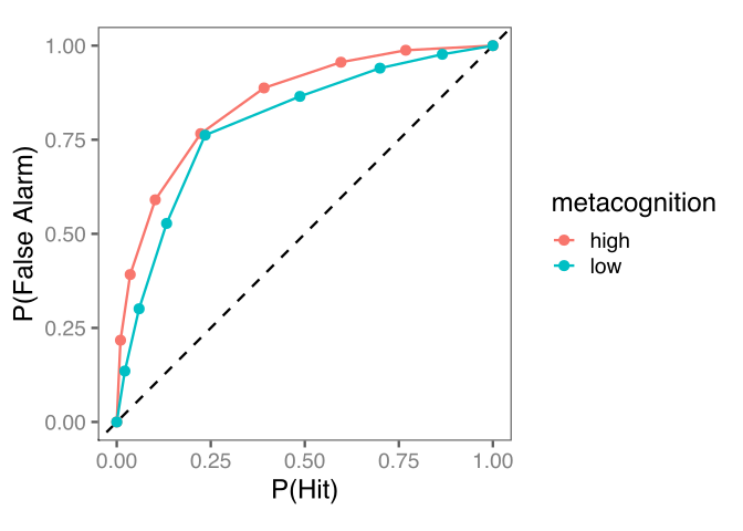
Similar to the type 2 ROCs we made above, we can also make pseudo type 1 ROCs by sliding a threshold from the left to the right of each histogram and taking the proportion of responses to the right of the threshold:
plot_roc1(d_metacognition, metacognition)Output
plot_roc1(d_performance, performance)Output
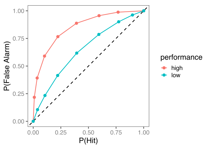
Although it was difficult to see before, these plots make it clear that there is indeed a difference: the type 1 ROC only changes shape with impaired metacognition, but it is drawn closer to the diagonal with reduced task performance! It is exactly this feature of the data that lets us distinguish changes in confidence ratings due to differences in metacognition from those due to differences in performance.
Understanding the meta-d’ model
Before we start model fitting, it will be helpful to have an idea of how the meta-d’ model captures metacognitive data. The model itself is split into two components, so we will go over each separately.
Note
If you are familiar with signal detection theory and the meta-d’ model, feel free to skip ahead!
Signal detection theory for type 1 responses
The meta-d’ model is built on one of the shining achievements of cognitive psychology: signal detection theory (Clarke et al. 1959). In a typical signal detection task, trials can be split up into one of four categories:
| Stimulus = 0 | Stimulus = 1 | |
|---|---|---|
| Response = 0 | Correct Rejection | Miss |
| Response = 1 | False Alarm | Hit |
For a stimulus S and response R, this lets us define four corresponding probabilities:
- P(\textrm{Hit}) = P(R=1 \vert S=1)
- P(\textrm{Miss}) = P(R=0 \vert S=1) = 1 - P(\textrm{Hit})
- P(\textrm{False Alarm}) = P(R=1 \vert S=0)
- P(\textrm{Correct Rejection}) = P(R=0 \vert S=0) = 1 - P(\textrm{False Alarm})
Our goal is to model these four probabilities. To do so, we will assume that people receive some noisy evidence about the stimulus, x_1. For simplicity, we will assume that the evidence has a normal distribution with a mean that depends on the stimulus S:
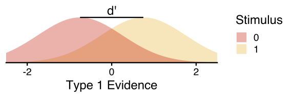
As the plot indicates, we’ll use d' to refer to the distance between the distributions of evidence for S=0 and S=1.
Then, we assume that people set an evidence threshold (or, criterion, c) that they use to decide whether they think S=0 or S=1. Specifically, people respond R=0 when the evidence is less than the threshold and R=1 when the evidence exceeds the threshold:
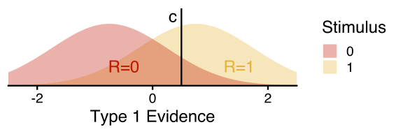
In this setup, the probability of a hit (alternatively, false alarm) is just the area under the yellow (alternatively, red) curve to the right of the threshold.
Modeling type 2 responses
The meta-d’ model adds to classical SDT by including a separate process for confidence ratings (Maniscalco and Lau 2012, 2014; Fleming 2017). This process works very similar: we assume that, depending on their previous response, people get another sample of noisy evidence about the stimulus to make confidence ratings (x_2), and then they threshold this evidence to make an confidence rating (C):
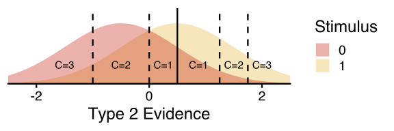
In this model, we refer to sensitivity of the evidence for confidence ratings as meta-d', the confidence criteria for zero responses as meta-c_2^0 and those for one responses as meta-c_2^1. Again, the probability of a confidence rating given a type 1 response is just the corresponding area under the red or yellow distribution curves.
ExerciseExercise: playing around with the meta-d’ model
To get a deeper understanding of how the model works, visit https://kevingoneill.shinyapps.io/hmetad to play around with the model and visualize the impact of its different parameters.2
Some things to think about while you explore:
- How does the shape of the ROC change as a function of metacognitive sensitivity? What does it look like at the extremes?
- How does the type 1 criterion (c) impact metacognition (type 2 ROC)? Does it impact metacognition equally for different type 1 responses?
- What happens when the type 2 criteria are close together? What kind of strategy might this reflect, cognitively?
AnswerSolution
- Metacognitive sensitivity affects the concavity of the type 1 ROC around its central point. When metacognitive sensitivity is optimal (meta-d' = d'), the type 1 ROC has a nice rounded shape defined by the normal distribution. When metacognitive sensitivity is low (meta-d' < d'), the type 1 ROC gets flatter, and becomes a perfect triangle when meta-d' = 0. Finally, when metacognitive sensitivity is high, the type 1 ROC takes an M-like shape, and forms three right angles as meta-d' \rightarrow\;\infty.
- The type 1 criterion determines which type 1 response is more likely overall. As a result, it makes metacognition easier for the response that becomes less likely, since more evidence is needed to make that response to begin with. For the same reason, it makes metacognition harder for the more common response.
- When the type 2 criteria are close together, the confidence rating between them becomes less likely and the higher confident ratings become more likely. This would correspond to a strategy with high metacognitive bias: the closer the type 2 criteria are, the less evidence is needed to make a confident response, and the more (over-)confident the person appears.
Fitting the meta-d’ model
Now that we have an idea about how models like the meta-d’ model can separate metacognitive sensitivity from type 1 performance, we can try fitting the model to some data! We will be using the hmetad package, which extends the original Hmetad-Toolbox in MATLAB (Fleming 2017).
Although we’ll be focusing on the meta-d’ model, we’ll try to take away some general lessons about Bayesian estimation. In particular, we’ll focus on two strategies used by Bayesian models to extract more precise and reliable estimates:
- Priors over model parameters bias inferences toward our expectations
- Hierarchical priors over participant-level parameters bias inferences about individual participants toward the population mean
Single-participant estimation
To start, let’s imagine we have data from just a single participant. To make things more realistic, we can simulate a new dataset with a smaller number of trials and a known set of parameters:
d <- sim_metad(
N_trials = 50, M = exp(-0.5),
dprime = 1.5, c = 0,
c2_0_diff = c(0.5, 0.5), c2_1_diff = c(0.5, 0.5)
)In order to fit the meta-d’ model, we first need to know which parameters the model has, since the number of confidence thresholds depends on the number of confidence levels in our data. To do so, we can use the following code:
metac2_parameters(K = 3)Output
[1] "metac2zero1diff" "metac2zero2diff" "metac2one1diff" "metac2one2diff" Because the data have three levels of confidence, our model will have two confidence thresholds for each type 1 response (the parameters are named with the suffix diff because, technically, they define the distances between thresholds). To fit our model, then, we simply call the fit_metad function with an R-style formula for each model parameter. For now, since we have only one participant and no covariates, we can model each parameter with just a fixed intercept (~ 1 in R formula syntax):
m <- fit_metad(
bf(
N ~ 1,
dprime ~ 1,
c ~ 1,
metac2zero1diff ~ 1,
metac2zero2diff ~ 1,
metac2one1diff ~ 1,
metac2one2diff ~ 1
),
data = d
)summary(m, prior = TRUE)Output
Family: metad__3__normal__absolute__multinomial
Links: mu = log; dprime = identity; c = identity; metac2zero1diff = log; metac2zero2diff = log; metac2one1diff = log; metac2one2diff = log
Formula: N ~ 1
dprime ~ 1
c ~ 1
metac2zero1diff ~ 1
metac2zero2diff ~ 1
metac2one1diff ~ 1
metac2one2diff ~ 1
Data: data.aggregated (Number of observations: 1)
Draws: 4 chains, each with iter = 2000; warmup = 1000; thin = 1;
total post-warmup draws = 4000
Priors:
Intercept ~ student_t(3, 0, 2.5)
Regression Coefficients:
Estimate Est.Error l-95% CI u-95% CI Rhat Bulk_ESS
Intercept -3.76 3.40 -12.93 -0.70 1.01 845
dprime_Intercept 2.19 0.45 1.34 3.08 1.00 2754
c_Intercept 0.08 0.22 -0.37 0.51 1.00 2377
metac2zero1diff_Intercept -0.89 0.35 -1.64 -0.25 1.00 2383
metac2zero2diff_Intercept -0.76 0.35 -1.54 -0.16 1.00 2583
metac2one1diff_Intercept -1.69 0.53 -2.83 -0.76 1.00 2392
metac2one2diff_Intercept -1.38 0.46 -2.41 -0.60 1.00 2289
Tail_ESS
Intercept 372
dprime_Intercept 2076
c_Intercept 2498
metac2zero1diff_Intercept 2691
metac2zero2diff_Intercept 1997
metac2one1diff_Intercept 2299
metac2one2diff_Intercept 1948
Draws were sampled using sampling(NUTS). For each parameter, Bulk_ESS
and Tail_ESS are effective sample size measures, and Rhat is the potential
scale reduction factor on split chains (at convergence, Rhat = 1).If we compare the model estimates of our parameters with their true values, we can see two patterns.
First, although the model estimates are close to the true values, they are not perfect.
ExerciseExercise
Why is this the case? To get an intuition, try re-running the data simulation and model fitting a couple of times to see how the results vary.
Second, our model estimates have a lot of uncertainty.
ExerciseExercise
Why might this happen?
Let’s dive into each of these questions individually.
Evaluating model fit with posterior retrodictive checks
We’ve already compared our model estimates with the ground truth parameter values used in our simulation. But it isn’t always easy to see how well a model captures the data just by looking at the parameter values.
To see things more clearly, we can compute the histograms and ROCs implied by the model, and compare those directly with the data. This process is called a posterior retrodictive check, because it uses the model posterior to make predictions of how it estimated the data to have looked. If the model retrodictions closely match the actual data, we can say that our model parameters describe these patterns well. If not, well, we have good reason to change something about our model.
For example, we can get the model predicted joint response probabilities using the function epred_draws_metad:
newdata <- tibble(participant = 1) ## a dataset to make predictions for
draws <- epred_draws_metad(m, newdata)
drawsOutput
Here, each row represents a single posterior sample, where .epred is the probability of a given type 1/type 2 response. Let’s plot these probabilities against the data:
plot_joint_response(d, draws = draws)Output
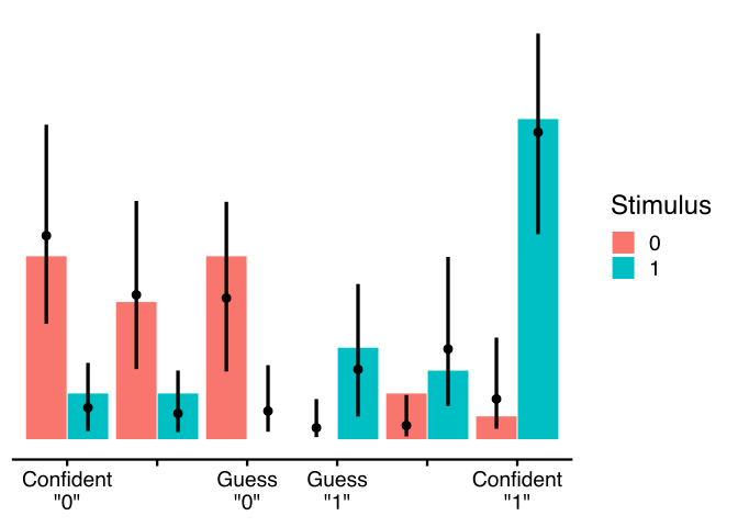
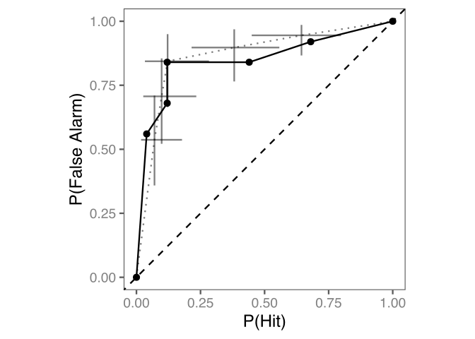
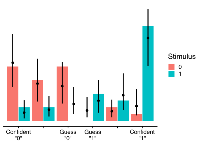
Even if our parameter estimates aren’t spot on, our prediction of the data is actually pretty good! If we like, we can also visualize the model predictions of the type 1 ROC in the same way:
plot_roc1(d, draws = roc1_draws(m, newdata, bounds = TRUE))Output
And the type 2 ROC:
plot_roc2(d, draws = roc2_draws(m, newdata, bounds = TRUE))Output
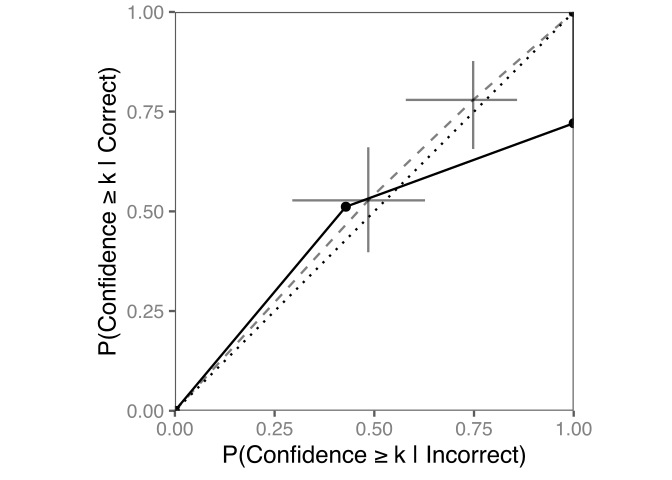
Similar to before, we can see that our model actually does a reasonable job of capturing the data, even if its predictions are not that precise.
Setting model priors with domain knowledge and prior prediction checks
Speaking of our model predictions being vague, why might this happen? There are actually two reasons. First, our dataset is somewhat small: with just 50 trials, we only get so much statistical power to fit this participant’s behavior. The other reason is that we have a lot of prior knowledge about metacognition that we aren’t yet incorporating into our model.
Let’s check the default priors used by our model:
prior_summary(m)Output
This table says that by default, brms put a wide t-distribution prior on \log(M), and no priors over the other parameters. This means that, before seeing the data, our model will allow d' to take literally any value: 0, -1, 100000, and -54321 are all considered equally likely! While all of these values are technically possible, if we actually estimated them in our data we would think that something went seriously wrong with our experiment—either the data was recorded improperly, the task was incredibly easy or difficuly, or the participants had a terrible misunderstanding of what they were supposed to do.
In Bayesian inference, we want to down-weight the probability of any of these crazy values from showing up. The way we do this is by specifying a prior distribution over each parameter that says which values we should expect in a typical experiment. There are two sources of information to help decide which priors to choose: (a) prior predictive checks and (b) domain knowledge.
A prior predictive check is just like the posterior retrodictive check we have already performed on our fitted model, except that (as the name suggests) we temporarily ignore the actual data and perform the check on our prior.
Important
Usually, one would perform a prior predictive check before collecting the data, since we should not let the data influence our choice of prior (that would be like Bayesian p-hacking!).
This means that one would normally not plot the data alongside the prior. But, for demonstration purposes, here we will plot the data as a comparison.
To start, let’s use really wide normal distributions for each parameter3
m_prior <- update(m,
sample_prior = "only",
prior = set_prior("normal(0, 5)", class = "Intercept") +
set_prior("normal(0, 5)",
class = "Intercept",
dpar = c("dprime", "c", metac2_parameters(K = 3))
)
)summary(m_prior)Output
Family: metad__3__normal__absolute__multinomial
Links: mu = log; dprime = identity; c = identity; metac2zero1diff = log; metac2zero2diff = log; metac2one1diff = log; metac2one2diff = log
Formula: N ~ 1
dprime ~ 1
c ~ 1
metac2zero1diff ~ 1
metac2zero2diff ~ 1
metac2one1diff ~ 1
metac2one2diff ~ 1
Data: data.aggregated (Number of observations: 1)
Draws: 4 chains, each with iter = 2000; warmup = 1000; thin = 1;
total post-warmup draws = 4000
Regression Coefficients:
Estimate Est.Error l-95% CI u-95% CI Rhat Bulk_ESS
Intercept 0.07 5.04 -9.70 9.79 1.00 5819
dprime_Intercept -0.13 4.93 -9.81 9.46 1.00 5479
c_Intercept -0.09 5.07 -9.91 9.75 1.00 4944
metac2zero1diff_Intercept 0.06 4.96 -9.58 9.66 1.00 5163
metac2zero2diff_Intercept -0.01 5.14 -9.94 10.02 1.00 5511
metac2one1diff_Intercept -0.06 5.01 -9.93 9.92 1.00 5977
metac2one2diff_Intercept -0.07 4.99 -9.87 9.48 1.00 5780
Tail_ESS
Intercept 3328
dprime_Intercept 2968
c_Intercept 3104
metac2zero1diff_Intercept 3217
metac2zero2diff_Intercept 2939
metac2one1diff_Intercept 3201
metac2one2diff_Intercept 3018
Draws were sampled using sampling(NUTS). For each parameter, Bulk_ESS
and Tail_ESS are effective sample size measures, and Rhat is the potential
scale reduction factor on split chains (at convergence, Rhat = 1).This model summary confirms that all of our parameters are just normal distributions with means of 0 (the Estimate column) and standard deviations of 5 (the Est.Error column). Now let’s plot our prior predicted probabilities:
plot_joint_response(d, draws = epred_draws_metad(m_prior, newdata))Output
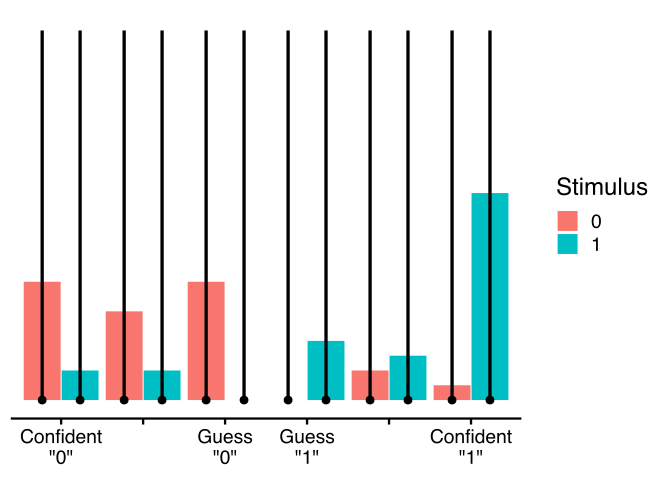
Well, that isn’t helpful. Since our prior is so wide, not only is every response expected to be equally likely, but each of the probabilities could be anything between 0 and 1. Clearly, something needs to change. But how do we decide what to change?
One strategy is trial and error: just pick a prior that feels right, simulate out its predictions, see what looks off, and iterate until you have something that you are happy with. Obviously this strategy will work, but it will likely take you some time.
ExerciseExercise: prior predictive checks
Try adjusting the prior in different ways. For each parameter, change the prior mean and/or the prior standard deviation. How does each of these change the prior predictions and posterior retrodictions?
AnswerSolution
When looking at the prior, setting the mean and standard deviation does what you might expect: it simply determines the relative weight we give to each parameter value.
In Bayesian inference, the posterior estimate will always be biased toward the prior mean. For example, if the prior mean is at M=1 but the M-ratio that makes the data most likely is M=\frac{1}{2}, the posterior mean will be somewhere between the two (M \in [\frac{1}{2}, 1]).
The prior standard deviation controls how strong this bias is. When the prior is wide, the bias is usually so small that the posterior will almost exactly match the most likely value. But when the prior is narrow, the posterior will look just like the prior even with a decently large dataset. Importantly, though, with enough data the posterior will always converge to the most likely value no matter how narrow the prior is.
A better strategy to start with, however, is to use whatever knowledge we happen to have about metacognition in general or our experiment in particular. For a typical psychological task, we would expect most M-ratios and d's to be roughly between 0.5 and 2, our cs to be roughly between -1 and 1, and the distances between confidence thresholds to be roughly between .1 and 5. So, let’s try again, setting normal priors that have roughly these ranges:
m_prior <- update(m,
sample_prior = "only",
prior = set_prior("normal(0, 0.5)", class = "Intercept") +
set_prior("normal(1, 0.5)", class = "Intercept", dpar = "dprime") +
set_prior("normal(0, 0.5)", class = "Intercept", dpar = "c") +
set_prior("normal(-0.5, 1)",
class = "Intercept",
dpar = metac2_parameters(K = 3)
)
)plot_joint_response(d, draws = epred_draws_metad(m_prior, newdata))Output
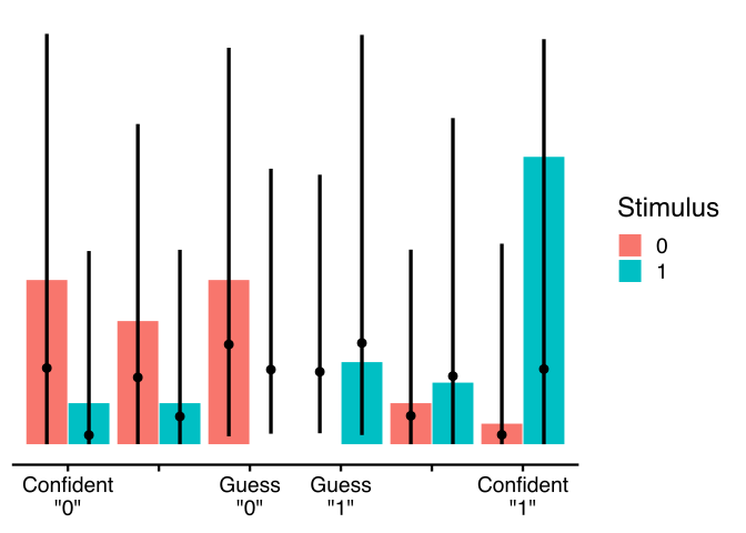
This prior still has a lot of uncertainty, but it is already looking much more reasonable: the prior probability of correct responses is higher than incorrect responses, and correct responses are more likely to be confident a priori. Of course, we might still want to tweak things a bit, but this is good enough for now.
Now let’s re-fit the model with our new priors:
m2 <- update(m_prior, sample_prior = "no")summary(m2)Output
Family: metad__3__normal__absolute__multinomial
Links: mu = log; dprime = identity; c = identity; metac2zero1diff = log; metac2zero2diff = log; metac2one1diff = log; metac2one2diff = log
Formula: N ~ 1
dprime ~ 1
c ~ 1
metac2zero1diff ~ 1
metac2zero2diff ~ 1
metac2one1diff ~ 1
metac2one2diff ~ 1
Data: data.aggregated (Number of observations: 1)
Draws: 4 chains, each with iter = 2000; warmup = 1000; thin = 1;
total post-warmup draws = 4000
Regression Coefficients:
Estimate Est.Error l-95% CI u-95% CI Rhat Bulk_ESS
Intercept -0.54 0.37 -1.29 0.13 1.00 4037
dprime_Intercept 1.55 0.32 0.95 2.18 1.00 5401
c_Intercept 0.02 0.18 -0.35 0.37 1.00 4427
metac2zero1diff_Intercept -0.75 0.32 -1.43 -0.19 1.00 5234
metac2zero2diff_Intercept -0.69 0.32 -1.37 -0.14 1.00 5228
metac2one1diff_Intercept -1.30 0.41 -2.17 -0.56 1.00 4415
metac2one2diff_Intercept -1.11 0.38 -1.93 -0.42 1.00 4905
Tail_ESS
Intercept 2573
dprime_Intercept 2880
c_Intercept 3146
metac2zero1diff_Intercept 2864
metac2zero2diff_Intercept 3414
metac2one1diff_Intercept 2895
metac2one2diff_Intercept 2938
Draws were sampled using sampling(NUTS). For each parameter, Bulk_ESS
and Tail_ESS are effective sample size measures, and Rhat is the potential
scale reduction factor on split chains (at convergence, Rhat = 1).Compared to our previous fit with flat priors, the parameter estimates are actually fairly similar! This is because our prior put relatively high probability over the true parameter values.
We can re-do our posterior retrodictive checks to see things more clearly:
plot_joint_response(d, draws = epred_draws_metad(m2, newdata))Output
plot_roc1(d, draws = roc1_draws(m2, newdata, bounds = TRUE))Output
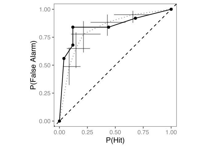
plot_roc2(d, draws = roc2_draws(m2, newdata, bounds = TRUE))Output
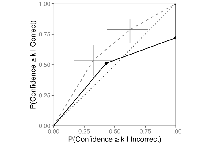
Compared to our estimates with flat priors, these model predictions are actually slightly further from the data, but they have less uncertainty.
ExerciseCheck your understanding
Why is this the case?
Is this a good or bad thing?
Try fitting the model again, but this time with really tight priors (e.g., set the prior standard deviations to 0.01).
How well does this model fit the data? Why?
AnswerSolution
Our model predictions are further away from the data and have less uncertainty because our new priors have a smaller width than our original flat priors. This sounds like a bad thing, but it is actually good: by forcing our estimates to be consistent with our prior knowledge, we are defending against the possibility that we obtain unexpected estimates simply by chance.
For example, our dataset above has no guesses (i.e., responses with minimal confidence). While we can tell that this participant tends to respond with high confidence, we don’t expect their guess rate to actually be zero. So, with a small dataset like this, we benefit from constraining how much the data can inform our inferences.
Hierarchical models for repeated measures
Until now we have been concerned with fitting data for a single participant. But most of the time we are interested in fitting data from many participants who vary in terms of how well they perform the task, how efficient their metacognition is, and how frequently they are to make different responses overall. So, we can decompose the trial-level variance into within-participant variance and between-participant variance. This strategy leads to a technique with many names: hierarchical modeling, linear mixed effects modeling, multilevel modeling.
Again, let’s start by simulating some data. Rather than set the parameters for each participant manually, we can simulate their parameters using a normal distribution. So, we simply need to define a mean and standard deviation for each parameter:
d <- sim_metad_participant(
N_participants = 10, N_trials = 50,
mean_M = -0.5, sd_M = 0.1,
mean_dprime = 1, sd_dprime = 0.1,
mean_c = 0, sd_c = 0.1,
mean_z_c2_0 = c(-0.5, -0.5), sd_z_c2_0 = c(0.25, 0.25), r_z_c2_0 = diag(2),
mean_z_c2_1 = c(-0.5, -0.5), sd_z_c2_1 = c(0.25, 0.25), r_z_c2_1 = diag(2)
) |>
mutate(participant = factor(participant))
dOutput
Single-participant estimation
Before we fit a hierarchical model, we can start by fitting each participant separately. For convenience, we’ll use the same priors as before, except now we will include a predictor for the participant number (using the R formula ~ 1 + participant) and put standard normal priors over the differences in parameters between participants.
# use sum-to-zero contrast coding
contrasts(d$participant) <- contr.sum
m_spe <- fit_metad(
bf(
N ~ 1 + participant,
dprime ~ 1 + participant,
c ~ 1 + participant,
metac2zero1diff ~ 1 + participant,
metac2zero2diff ~ 1 + participant,
metac2one1diff ~ 1 + participant,
metac2one2diff ~ 1 + participant
),
data = d, init = 0,
prior = set_prior("normal(0, 0.5)", class = "Intercept") +
set_prior("normal(1, 0.5)", class = "Intercept", dpar = "dprime") +
set_prior("normal(0, 0.5)", class = "Intercept", dpar = "c") +
set_prior("normal(-0.5, 1)",
class = "Intercept",
dpar = metac2_parameters(K = 3)
) +
set_prior("normal(0, 1)", class = "b") +
set_prior("normal(0, 1)", class = "b", dpar = c("dprime", "c", metac2_parameters(K = 3)))
)summary(m_spe)Output
Family: metad__3__normal__absolute__multinomial
Links: mu = log; dprime = identity; c = identity; metac2zero1diff = log; metac2zero2diff = log; metac2one1diff = log; metac2one2diff = log
Formula: N ~ 1 + participant
dprime ~ 1 + participant
c ~ 1 + participant
metac2zero1diff ~ 1 + participant
metac2zero2diff ~ 1 + participant
metac2one1diff ~ 1 + participant
metac2one2diff ~ 1 + participant
Data: data.aggregated (Number of observations: 10)
Draws: 4 chains, each with iter = 2000; warmup = 1000; thin = 1;
total post-warmup draws = 4000
Regression Coefficients:
Estimate Est.Error l-95% CI u-95% CI Rhat Bulk_ESS
Intercept -0.85 0.30 -1.47 -0.31 1.00 3560
dprime_Intercept 1.11 0.11 0.89 1.33 1.00 6591
c_Intercept -0.02 0.06 -0.14 0.09 1.00 4139
metac2zero1diff_Intercept -0.53 0.10 -0.72 -0.35 1.00 4457
metac2zero2diff_Intercept -0.62 0.12 -0.87 -0.38 1.00 5422
metac2one1diff_Intercept -0.67 0.10 -0.87 -0.47 1.00 4338
metac2one2diff_Intercept -0.48 0.11 -0.70 -0.28 1.00 4890
participant1 -0.47 0.68 -1.89 0.75 1.00 5082
participant2 0.17 0.64 -1.30 1.26 1.00 3324
participant3 0.44 0.78 -1.24 1.87 1.00 4245
participant4 0.46 0.62 -0.98 1.55 1.00 2832
participant5 0.27 0.77 -1.39 1.68 1.00 4605
participant6 -0.02 0.68 -1.48 1.17 1.00 3958
participant7 -0.02 0.79 -1.60 1.48 1.00 5225
participant8 0.13 0.74 -1.42 1.51 1.00 4587
participant9 -0.26 0.64 -1.62 0.93 1.00 4320
dprime_participant1 0.08 0.34 -0.57 0.77 1.00 6083
dprime_participant2 0.38 0.34 -0.29 1.05 1.00 5502
dprime_participant3 -0.49 0.29 -1.05 0.09 1.00 5418
dprime_participant4 0.28 0.33 -0.37 0.95 1.00 5664
dprime_participant5 -0.34 0.32 -0.96 0.28 1.00 5802
dprime_participant6 0.25 0.34 -0.38 0.93 1.00 5896
dprime_participant7 -0.52 0.32 -1.14 0.13 1.00 6130
dprime_participant8 -0.27 0.32 -0.89 0.34 1.00 5861
dprime_participant9 0.23 0.35 -0.45 0.91 1.00 6431
c_participant1 -0.14 0.18 -0.48 0.20 1.00 4430
c_participant2 0.08 0.18 -0.30 0.44 1.00 4854
c_participant3 0.12 0.17 -0.22 0.45 1.00 3865
c_participant4 0.05 0.18 -0.29 0.39 1.00 3863
c_participant5 -0.15 0.17 -0.48 0.19 1.00 4103
c_participant6 0.15 0.17 -0.19 0.50 1.00 4136
c_participant7 -0.02 0.17 -0.36 0.32 1.00 4360
c_participant8 0.08 0.17 -0.24 0.41 1.00 4666
c_participant9 -0.11 0.18 -0.46 0.23 1.00 4368
metac2zero1diff_participant1 0.16 0.25 -0.34 0.64 1.00 5198
metac2zero1diff_participant2 -0.10 0.28 -0.70 0.43 1.00 4762
metac2zero1diff_participant3 0.31 0.22 -0.15 0.72 1.00 4765
metac2zero1diff_participant4 -0.18 0.31 -0.84 0.39 1.00 4649
metac2zero1diff_participant5 -1.08 0.41 -1.96 -0.35 1.00 3710
metac2zero1diff_participant6 0.05 0.27 -0.51 0.55 1.00 4536
metac2zero1diff_participant7 0.71 0.21 0.30 1.11 1.00 4713
metac2zero1diff_participant8 0.27 0.23 -0.21 0.70 1.00 4313
metac2zero1diff_participant9 0.04 0.26 -0.50 0.52 1.00 5370
metac2zero2diff_participant1 0.23 0.34 -0.48 0.84 1.00 5246
metac2zero2diff_participant2 0.62 0.25 0.12 1.08 1.00 5429
metac2zero2diff_participant3 -0.15 0.35 -0.87 0.46 1.00 5959
metac2zero2diff_participant4 0.58 0.27 0.03 1.08 1.00 5668
metac2zero2diff_participant5 -0.25 0.33 -0.93 0.35 1.00 5253
metac2zero2diff_participant6 -0.30 0.35 -1.04 0.33 1.00 5469
metac2zero2diff_participant7 -0.15 0.45 -1.14 0.63 1.00 5439
metac2zero2diff_participant8 0.41 0.30 -0.22 0.97 1.00 6934
metac2zero2diff_participant9 -0.16 0.35 -0.91 0.47 1.00 6309
metac2one1diff_participant1 0.44 0.22 -0.02 0.85 1.00 4554
metac2one1diff_participant2 0.15 0.28 -0.44 0.68 1.00 4876
metac2one1diff_participant3 -0.06 0.29 -0.64 0.47 1.00 5120
metac2one1diff_participant4 0.14 0.28 -0.41 0.65 1.00 4704
metac2one1diff_participant5 0.07 0.26 -0.47 0.55 1.00 4650
metac2one1diff_participant6 -0.25 0.32 -0.93 0.35 1.00 4653
metac2one1diff_participant7 0.42 0.23 -0.06 0.86 1.00 5117
metac2one1diff_participant8 0.32 0.24 -0.17 0.76 1.00 4367
metac2one1diff_participant9 -0.56 0.36 -1.34 0.09 1.00 5462
metac2one2diff_participant1 0.34 0.27 -0.22 0.83 1.00 5845
metac2one2diff_participant2 0.19 0.29 -0.42 0.73 1.00 4840
metac2one2diff_participant3 -0.21 0.32 -0.88 0.36 1.00 5527
metac2one2diff_participant4 0.56 0.26 0.04 1.05 1.00 5185
metac2one2diff_participant5 0.12 0.27 -0.44 0.63 1.00 5581
metac2one2diff_participant6 -0.29 0.32 -0.95 0.29 1.00 5247
metac2one2diff_participant7 -0.43 0.37 -1.24 0.22 1.00 5482
metac2one2diff_participant8 -0.20 0.34 -0.89 0.41 1.00 5563
metac2one2diff_participant9 0.23 0.24 -0.27 0.67 1.00 5441
Tail_ESS
Intercept 3291
dprime_Intercept 3221
c_Intercept 3214
metac2zero1diff_Intercept 3300
metac2zero2diff_Intercept 2892
metac2one1diff_Intercept 3316
metac2one2diff_Intercept 3050
participant1 3531
participant2 2917
participant3 3160
participant4 2434
participant5 2889
participant6 2767
participant7 2946
participant8 3148
participant9 3290
dprime_participant1 2943
dprime_participant2 2704
dprime_participant3 3185
dprime_participant4 3041
dprime_participant5 3003
dprime_participant6 2916
dprime_participant7 3146
dprime_participant8 3301
dprime_participant9 3100
c_participant1 3067
c_participant2 3621
c_participant3 2974
c_participant4 3199
c_participant5 3408
c_participant6 2931
c_participant7 3003
c_participant8 3296
c_participant9 3473
metac2zero1diff_participant1 3044
metac2zero1diff_participant2 2970
metac2zero1diff_participant3 3762
metac2zero1diff_participant4 3101
metac2zero1diff_participant5 2904
metac2zero1diff_participant6 2969
metac2zero1diff_participant7 2485
metac2zero1diff_participant8 2889
metac2zero1diff_participant9 3357
metac2zero2diff_participant1 3010
metac2zero2diff_participant2 2963
metac2zero2diff_participant3 2642
metac2zero2diff_participant4 3057
metac2zero2diff_participant5 2734
metac2zero2diff_participant6 2234
metac2zero2diff_participant7 2924
metac2zero2diff_participant8 3010
metac2zero2diff_participant9 2901
metac2one1diff_participant1 3114
metac2one1diff_participant2 2640
metac2one1diff_participant3 3109
metac2one1diff_participant4 3155
metac2one1diff_participant5 2959
metac2one1diff_participant6 2313
metac2one1diff_participant7 3363
metac2one1diff_participant8 3056
metac2one1diff_participant9 3245
metac2one2diff_participant1 2992
metac2one2diff_participant2 2814
metac2one2diff_participant3 2537
metac2one2diff_participant4 2832
metac2one2diff_participant5 3094
metac2one2diff_participant6 2781
metac2one2diff_participant7 2834
metac2one2diff_participant8 2796
metac2one2diff_participant9 3193
Draws were sampled using sampling(NUTS). For each parameter, Bulk_ESS
and Tail_ESS are effective sample size measures, and Rhat is the potential
scale reduction factor on split chains (at convergence, Rhat = 1).Because we used sum-to-zero contrast coding for participants, our model has two sets of parameters. The Intercept parameters reflect the average values across all participants, and the participantX parameters reflect the difference between the group average and participant X. Despite breaking our parameters down into group averages and between-participant differences, however, the parameter estimates for each participant are estimated independently.
We can plot the estimated type 1 ROCs for each participant:
newdata <- distinct(d, participant)
plot_roc1(d, participant, draws = roc1_draws(m_spe, newdata)) +
facet_wrap(~participant)Output
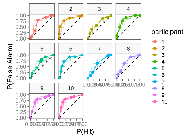
On first glance, this looks really good! The model predictions are very close to the data, so what could possibly be wrong?
To get an idea, let’s resimulate our data from the same participants with the same ground truth parameter values.
d2 <- resimulate(d)
m_spe2 <- update(m_spe, newdata = aggregate_metad(d2, participant))plot_roc1(d2, participant, draws = roc1_draws(m_spe2, newdata)) +
facet_wrap(~participant)Output
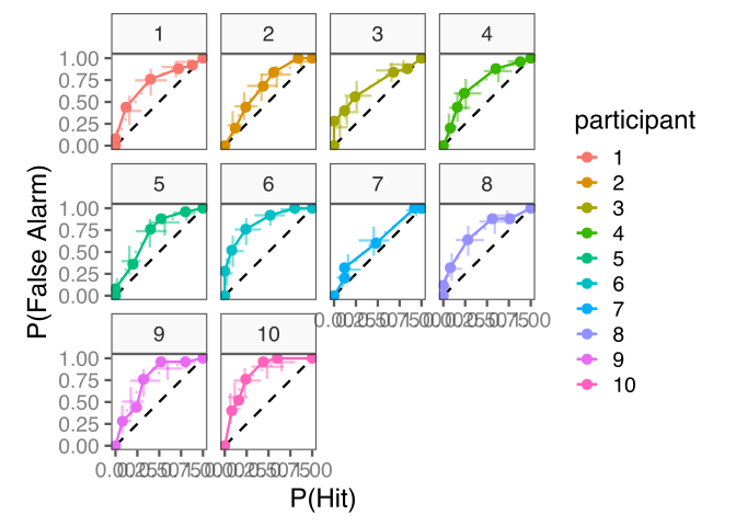
If you flip back and forth between the two datasets, what stands out to you?
Even though both datasets have the same ground truth parameters, they look very different from one another! Moreover, the model fits the data very well in both cases. Again, this might sound like a good thing, but it’s actually not what we want. Of course we want the model to fit our data. But more importantly, we want the parameter estimates for each participant to be as close as possible to their ground truth values. In other words, we want the estimates that we would get if we were able to collect an infinite number of trials per participant. Since we only have a small number of trials per participant, and since metacognition is noisy, we can only trust the data from any given participant so much. This is Stein’s paradox: the best estimate of a participant’s parameters doesn’t just use their data, but instead uses the data from all participants!
The solution is for each participant’s estimates to strike a balance between their empirical values and the average across all participants (sound familiar?). We can achieve this by explicitly modeling the variability between participants.
Hierarchical estimation
To fit the hierarchical (or multilevel) version of the model, we only need to make two changes. First, rather than simply having a coefficient for participant, we can set participant as a grouping factor using the syntax ~ 1 + (1 | participant), which will result in an intercept representing the group mean and an offset from the group mean for each participant. Second, instead of setting a prior directly on the differences between participants, we set a prior on the standard deviation of those differences:
m_he <- fit_metad(
bf(
N ~ 1 + (1 | participant),
dprime ~ 1 + (1 | participant),
c ~ 1 + (1 | participant),
metac2zero1diff ~ 1 + (1 | participant),
metac2zero2diff ~ 1 + (1 | participant),
metac2one1diff ~ 1 + (1 | participant),
metac2one2diff ~ 1 + (1 | participant)
),
data = d, init = 0,
prior = set_prior("normal(0, 0.5)", class = "Intercept") +
set_prior("normal(1, 0.5)", class = "Intercept", dpar = "dprime") +
set_prior("normal(0, 0.5)", class = "Intercept", dpar = "c") +
set_prior("normal(-0.5, 1)",
class = "Intercept",
dpar = metac2_parameters(K = 3)
) +
set_prior("normal(0, 1)", class = "sd") +
set_prior("normal(0, 1)", class = "sd", dpar = c("dprime", "c", metac2_parameters(K = 3)))
)summary(m_he)Output
Family: metad__3__normal__absolute__multinomial
Links: mu = log; dprime = identity; c = identity; metac2zero1diff = log; metac2zero2diff = log; metac2one1diff = log; metac2one2diff = log
Formula: N ~ 1 + (1 | participant)
dprime ~ 1 + (1 | participant)
c ~ 1 + (1 | participant)
metac2zero1diff ~ 1 + (1 | participant)
metac2zero2diff ~ 1 + (1 | participant)
metac2one1diff ~ 1 + (1 | participant)
metac2one2diff ~ 1 + (1 | participant)
Data: data.aggregated (Number of observations: 10)
Draws: 4 chains, each with iter = 2000; warmup = 1000; thin = 1;
total post-warmup draws = 4000
Multilevel Hyperparameters:
~participant (Number of levels: 10)
Estimate Est.Error l-95% CI u-95% CI Rhat
sd(Intercept) 0.34 0.28 0.01 1.03 1.00
sd(dprime_Intercept) 0.25 0.16 0.01 0.62 1.00
sd(c_Intercept) 0.06 0.05 0.00 0.20 1.00
sd(metac2zero1diff_Intercept) 0.40 0.18 0.11 0.81 1.00
sd(metac2zero2diff_Intercept) 0.34 0.19 0.03 0.75 1.00
sd(metac2one1diff_Intercept) 0.29 0.16 0.03 0.65 1.00
sd(metac2one2diff_Intercept) 0.20 0.15 0.01 0.57 1.00
Bulk_ESS Tail_ESS
sd(Intercept) 2405 2237
sd(dprime_Intercept) 1519 2084
sd(c_Intercept) 2630 2279
sd(metac2zero1diff_Intercept) 1079 1123
sd(metac2zero2diff_Intercept) 953 998
sd(metac2one1diff_Intercept) 1244 1385
sd(metac2one2diff_Intercept) 1351 1886
Regression Coefficients:
Estimate Est.Error l-95% CI u-95% CI Rhat Bulk_ESS
Intercept -0.54 0.28 -1.13 -0.03 1.00 5357
dprime_Intercept 1.08 0.14 0.81 1.37 1.00 4649
c_Intercept -0.02 0.06 -0.15 0.11 1.00 7206
metac2zero1diff_Intercept -0.47 0.16 -0.82 -0.17 1.00 2729
metac2zero2diff_Intercept -0.54 0.16 -0.89 -0.24 1.00 3686
metac2one1diff_Intercept -0.60 0.14 -0.89 -0.34 1.00 3833
metac2one2diff_Intercept -0.43 0.13 -0.69 -0.19 1.00 4545
Tail_ESS
Intercept 3014
dprime_Intercept 3056
c_Intercept 3082
metac2zero1diff_Intercept 2747
metac2zero2diff_Intercept 2534
metac2one1diff_Intercept 2999
metac2one2diff_Intercept 2411
Draws were sampled using sampling(NUTS). For each parameter, Bulk_ESS
and Tail_ESS are effective sample size measures, and Rhat is the potential
scale reduction factor on split chains (at convergence, Rhat = 1).You can immediately see that this model output is a lot easier to read than the earlier one. It’s separated into two sections: Multilevel Hyperparameters, which contains the estimates of the variability in parameters between participants, and Regression Coefficients, which in this case just shows the average parameter values across participants. But don’t let that fool you—this model also contains estimates for each participant.
plot_roc1(d, participant, draws = roc1_draws(m_he, newdata)) +
facet_wrap(~participant)Output
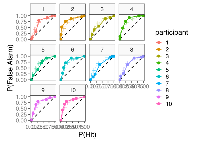
This model also makes it easy to obtain predictions averaging across participants:
plot_roc1(d, draws = roc1_draws(m_he, tibble(.row = 1), re_formula = NA))Output
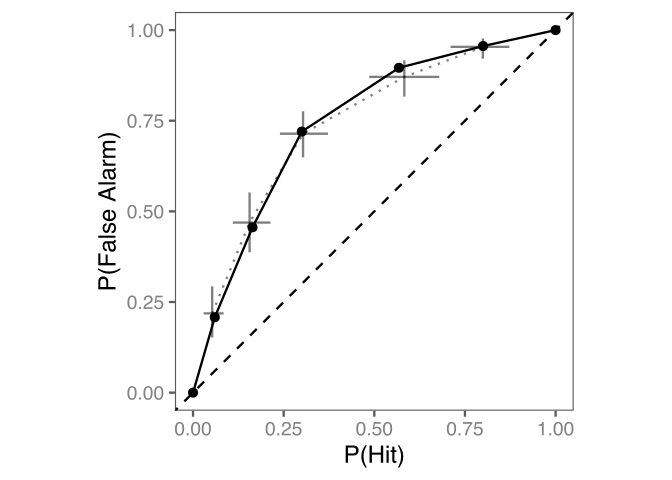
Compared to the model with independent estimates for each participant, this model seems to fit the data less well. In particular, the ROCs (and estimated parameters) for each participant are shrunk toward the group average. This effect—known as partial pooling—is notably stronger for outlier participants. To show that this really is a good thing, let’s re-fit the hierarchical model to the resimulated data:
m_he2 <- update(m_he, newdata = aggregate_metad(d2, participant))
plot_roc1(d2, participant, draws = roc1_draws(m_he2, newdata)) +
facet_wrap(~participant)Output
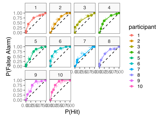
This time, even though the data for each participant looks very different from the last sample, our participant-level estimates actually look quite similar! This is the magic of hierchical models: by carefully separating within-participant and between-participant variance, we can actually obtain better parameter estimates by fitting the data less well!
Key takeaways
We started with the goal of better understanding metacognition is measured and how it is modeled in a Bayesian framework. We covered a lot, but if you take anything away with you from this tutorial, let it be this:
- Researchers aim to construct and use measures of metacognitive sensitivity (i.e., how well confidence tracks accuracy) and metacognitive bias (i.e., how confident one is overall).
- Measures of metacognition need to account for first-order performance, since apparent differences in confidence ratings are expected to arise from differences in performance.
- Bayesian inference uses informed priors to help constrain models like the meta-d' model. This often results in a less good fit of the data, but better estimates in the long run.
- Hierarchical models constrain participant-level parameter estimates across participants by assuming that, a priori, participants should behave somewhat like each other.
If you have some extra time, continue on to take a deeper dive into how to interpret your model’s posterior distributions!
Extension 1: posterior wrangling
So far, we have simply fit some models to simulated data, inspected the model summaries, and plotted the posterior distributions. But how do we actually extract a model’s (prior or) posterior distribution and do anything with it?
To do this, the tidybayes package is your friend—it provides really convenient functions to manipulate your posterior distributions. In fact, it is so useful that hmetad includes several functions we have already used that are modeled exactly on the tidybayes package! Throughout, we’ll use the existing hierarchical model as an example.
The tidybayes package has three main functions for obtaining three kinds of model outputs:
linpred_draws: obtain samples of the posterior distribution over model parameters (M-ratio, d', etc)epred_draws: obtain samples of the posterior distribution over the predicted probabilities (i.e., expectation of the posterior predictive distribution)predicted_draws: obtain samples of the posterior distribution over the data (i.e., the posterior predictive distribution)
Obtaining model parameters
Let’s start with linpred_draws, which takes a model object and a dataset for which to make predictions:
linpred_draws(m_he, newdata)Output
As you can see, here we have a dataset with one row per posterior sample (called a draw) and per row of newdata (here, per participant). By default, linpred_draws only returns samples of the main model parameter on its latent scale, which for hmetad means that the column .linpred contains samples of \log(M).
If you would like the parameters returned on their true scale (i.e., M instead of \log(M)), you can set transform=TRUE:
linpred_draws(m_he, newdata, transform = TRUE)Output
If you would like other parameters as well, you can include them using the dpar argument:
linpred_draws(m_he, newdata, dpar = c("dprime", "c"))Output
Since it can be tedious to remember all of these arguments, the hmetad package includes the function linpred_draws_metad, which returns all model parameters on their true scale:
linpred_draws_metad(m_he, newdata)Output
Finally, the re_formula argument controls which hierarchical parameters (or random effects) are included in the returned output. By default, all tidybayes functions will use all hierarchical parameters, which in this case means that it makes unique predictions for each participant. We can ignore participant-level differences by setting re_formula=NA. For instance, to obtain the mean parameter estimates across all participants, we can do this:
linpred_draws_metad(m_he, tibble(.row = 1), re_formula = NA)Output
Metacognitive bias
These functions work really well for just obtaining predictions of the model parameters themselves, which give us good measures of metacognitive efficiency, type 1 sensitivity, and type 1 response bias. But you might have noticed that there are a number of different confidence criteria, making it complicated to determine a participants’ metacognitive bias (i.e., their overall level of confidence). Instead of interpreting all of these confidence criteria separately, we now recommmend computing a derived measure called meta-\Delta:
metacognitive_bias_draws(m_he, newdata)Output
This gives us a separate measure of metacognitive bias for each type 1 response (indicated by the response column). We do this to account for possible differences in confidence for the two responses (e.g., in a detection task a participant might be over-confident in “present” responses but under-confident in “absent” responses). If we want just a single number averaged over both responses, we can set the argument by_response=FALSE:
metacognitive_bias_draws(m_he, newdata, by_response = FALSE)Output
Note that these measures are defined in standardized units, such that 0 represents a participant that always responds with the highest level of confidence and \infty represents a participant that always responds with the lowest level of confidence.
Obtaining posterior summaries
Of course it can be helpful to have a tidy dataset containing all of our posterior draws. But we will almost always want to summarize our posterior to share our results with others. In particular, we will want a measure of central tendency (i.e., mean, median, or mode) and some measure of uncertainty (i.e., posterior quantiles or highest density intervals). To get any of these, tidybayes includes a function named [point]_[interval]. For example, to get posterior medians and 95% quantiles, we can use median_qi:
linpred_draws_metad(m_he, tibble(.row = 1), re_formula = NA) |>
median_qi()Output
Alternatively, for an easier-to-read output, we can use the pivot_longer argument to linpred_draws_metad and then explicitly name the column to summarize in median_qi:
linpred_draws_metad(m_he, tibble(.row = 1), re_formula = NA, pivot_longer = TRUE) |>
median_qi(.value)Output
Yet another alternative is, instead of the _draws functions, to use the _rvar variant, which only has one row for the full posterior and displays the posterior mean and standard deviation by default:
linpred_rvars_metad(m_he, tibble(.row = 1), re_formula = NA, pivot_longer = TRUE)Output
Obtaining predicted probabilities
The next kind of posterior we would like is a posterior over the predicted probabilities of the type 1 and type 2 responses, which can be obtained using epred_draws. Thankfully, this works just like the linpred_draws function:
epred_draws(m_he, newdata) |>
median_qi(.epred)Output
Here, the .epred column contains the probability that a given participant makes a given response with a given level of confidence for a given stimulus. For models fitted with hmetad, this is not incredibly helpful because it includes a single column .category which labels the stimulus and the joint type 1/type 2 response. To get a more useful output, we can use epred_draws_metad:
epred_draws_metad(m_he, newdata) |>
median_qi(.epred)Output
As we have already seen in the tutorial above, this is very useful for doing prior predictive checks and posterior retrodictive checks to assess the suitability of your prior and model for describing the data. But there are a host of other kinds of model predictions that we can compute using these predicted probabilities!
Mean confidence
First, if we know the probability of a given type 1 and type 2 response, we can compute model predictions of mean confidence4:
mean_confidence_draws(m_he, newdata) |>
median_qi(.epred)Output
Conveniently, this provides estimates of mean confidence on the actual confidence scale used by participants. By default, this gives us a separate prediction for each stimulus and each type 1 response. If we like, we can also make predictions averaging over stimulus (by_stimulus=FALSE), responses (by_response=FALSE), or both:
mean_confidence_draws(m_he, newdata, by_stimulus = FALSE, by_response = FALSE) |>
median_qi(.epred)Output
Finally, we can also get predictions by accuracy as a data-driven index of metacognitive sensitivity5:
mean_confidence_draws(m_he, newdata, by_correct = TRUE) |>
median_qi(.epred)Output
Receiver operating characteristic curves
As we have already seen above, we can also use similar functions to get the type 1 ROC:
roc1_draws(m_he, newdata) |>
median_qi(p_hit, p_fa)Output
And the type 2 ROC:
roc2_draws(m_he, newdata) |>
median_qi(p_hit2, p_fa2)Output
Obtaining simulated data
The last kind of posterior distribution we can obtain is a posterior over simulated data. That is, given our fitted model parameters (and our uncertainty in them), we can directly simulate data with the predicted_draws function. Importantly, to use this function, we need to include a column N in newdata which represents the number of trials to simulate:
newdata |>
mutate(N = 100) |>
predicted_draws(m_he, newdata = _) |>
median_qi(.prediction)Output
In this output, the .prediction column contains the simulated number of trials with the corresponding stimulus and type 1/type 2 response. As with epred_draws, it is usually more convenient to use the corresponding hmetad function predicted_draws_metad:
newdata |>
mutate(N = 100) |>
predicted_draws_metad(m_he, newdata = _) |>
median_qi(.prediction)Output
We won’t go into more details here, but being able to simulate data in this way is critical for performing simulation-based power analyses to detect the required sample size (number of participants, trials, stimuli, etc) for a given effect size of interest.
Wrapping up
That is a lot of different quantities that we can extract from our model! Of course, it is usually not necessary to investigate all of these outputs. Instead, it is usually best to pick a small number of measures that answer your key research questions.
Thankfully, regardless of which measure you are interested in, the hmetad package provides a common interface to extract your model’s predictions.
Extension 2: significance testing
Now that we know how to get model predictions, the last thing we will likely need to do in a research project is to compare our model predictions under different conditions.
To demonstrate this, we will require a dataset with within-participant conditions:
d <- sim_metad_participant_condition(
N_participants = 20, N_trials = 200,
mean_M = c(0, -1)
) |>
mutate(condition = factor(condition))
dOutput
Next, we’ll fit another hierarchical model, but this time with group-level and participant-level effects of condition6 (note that this model will likely take some time to fit):
m <- fit_metad(
bf(
N ~ condition + (condition | participant),
dprime ~ condition + (condition | participant),
c ~ condition + (condition | participant),
metac2zero1diff ~ condition + (condition | participant),
metac2zero2diff ~ condition + (condition | participant),
metac2zero3diff ~ condition + (condition | participant),
metac2one1diff ~ condition + (condition | participant),
metac2one2diff ~ condition + (condition | participant),
metac2one3diff ~ condition + (condition | participant)
),
data = d, init = 0,
prior = set_prior("normal(0, 0.5)", class = "Intercept") +
set_prior("normal(1, 0.5)", class = "Intercept", dpar = "dprime") +
set_prior("normal(0, 0.5)", class = "Intercept", dpar = "c") +
set_prior("normal(-0.5, 1)",
class = "Intercept",
dpar = metac2_parameters(K = 4)
) +
set_prior("normal(0, 1)", class = "b") +
set_prior("normal(0, 1)", class = "b", dpar = c("dprime", "c", metac2_parameters(K = 4))) +
set_prior("normal(0, 1)", class = "sd") +
set_prior("normal(0, 1)", class = "sd", dpar = c("dprime", "c", metac2_parameters(K = 4)))
)
summary(m)Output
0.03 1.05
sd(dprime_Intercept) 0.37 0.76
sd(dprime_condition2) 0.51 1.05
sd(c_Intercept) 0.39 0.75
sd(c_condition2) 0.50 0.96
sd(metac2zero1diff_Intercept) 0.00 0.15
sd(metac2zero1diff_condition2) 0.01 0.30
sd(metac2zero2diff_Intercept) 0.00 0.23
sd(metac2zero2diff_condition2) 0.03 0.42
sd(metac2zero3diff_Intercept) 0.00 0.16
sd(metac2zero3diff_condition2) 0.00 0.31
sd(metac2one1diff_Intercept) 0.00 0.24
sd(metac2one1diff_condition2) 0.01 0.36
sd(metac2one2diff_Intercept) 0.00 0.21
sd(metac2one2diff_condition2) 0.00 0.18
sd(metac2one3diff_Intercept) 0.01 0.30
sd(metac2one3diff_condition2) 0.00 0.31
cor(Intercept,condition2) -0.97 0.73
cor(dprime_Intercept,dprime_condition2) -0.92 -0.46
cor(c_Intercept,c_condition2) -0.87 -0.36
cor(metac2zero1diff_Intercept,metac2zero1diff_condition2) -0.98 0.90
cor(metac2zero2diff_Intercept,metac2zero2diff_condition2) -0.99 0.80
cor(metac2zero3diff_Intercept,metac2zero3diff_condition2) -0.98 0.92
cor(metac2one1diff_Intercept,metac2one1diff_condition2) -0.98 0.85
cor(metac2one2diff_Intercept,metac2one2diff_condition2) -0.97 0.91
cor(metac2one3diff_Intercept,metac2one3diff_condition2) -0.99 0.88
Rhat Bulk_ESS
sd(Intercept) 1.00 1716
sd(condition2) 1.00 1629
sd(dprime_Intercept) 1.00 1544
sd(dprime_condition2) 1.00 1446
sd(c_Intercept) 1.00 950
sd(c_condition2) 1.00 1097
sd(metac2zero1diff_Intercept) 1.00 2477
sd(metac2zero1diff_condition2) 1.00 1307
sd(metac2zero2diff_Intercept) 1.00 1349
sd(metac2zero2diff_condition2) 1.00 739
sd(metac2zero3diff_Intercept) 1.00 2447
sd(metac2zero3diff_condition2) 1.00 1477
sd(metac2one1diff_Intercept) 1.00 1251
sd(metac2one1diff_condition2) 1.00 878
sd(metac2one2diff_Intercept) 1.00 1399
sd(metac2one2diff_condition2) 1.00 2589
sd(metac2one3diff_Intercept) 1.00 1361
sd(metac2one3diff_condition2) 1.00 1479
cor(Intercept,condition2) 1.00 3621
cor(dprime_Intercept,dprime_condition2) 1.00 1191
cor(c_Intercept,c_condition2) 1.00 1086
cor(metac2zero1diff_Intercept,metac2zero1diff_condition2) 1.00 1846
cor(metac2zero2diff_Intercept,metac2zero2diff_condition2) 1.01 784
cor(metac2zero3diff_Intercept,metac2zero3diff_condition2) 1.00 2726
cor(metac2one1diff_Intercept,metac2one1diff_condition2) 1.00 1484
cor(metac2one2diff_Intercept,metac2one2diff_condition2) 1.00 4064
cor(metac2one3diff_Intercept,metac2one3diff_condition2) 1.00 2658
Tail_ESS
sd(Intercept) 2359
sd(condition2) 2091
sd(dprime_Intercept) 2432
sd(dprime_condition2) 1891
sd(c_Intercept) 1758
sd(c_condition2) 1778
sd(metac2zero1diff_Intercept) 2614
sd(metac2zero1diff_condition2) 2361
sd(metac2zero2diff_Intercept) 1930
sd(metac2zero2diff_condition2) 972
sd(metac2zero3diff_Intercept) 2550
sd(metac2zero3diff_condition2) 2047
sd(metac2one1diff_Intercept) 1966
sd(metac2one1diff_condition2) 1271
sd(metac2one2diff_Intercept) 1388
sd(metac2one2diff_condition2) 1962
sd(metac2one3diff_Intercept) 1546
sd(metac2one3diff_condition2) 2135
cor(Intercept,condition2) 2998
cor(dprime_Intercept,dprime_condition2) 2046
cor(c_Intercept,c_condition2) 1761
cor(metac2zero1diff_Intercept,metac2zero1diff_condition2) 2624
cor(metac2zero2diff_Intercept,metac2zero2diff_condition2) 1482
cor(metac2zero3diff_Intercept,metac2zero3diff_condition2) 2982
cor(metac2one1diff_Intercept,metac2one1diff_condition2) 2098
cor(metac2one2diff_Intercept,metac2one2diff_condition2) 2668
cor(metac2one3diff_Intercept,metac2one3diff_condition2) 2830
Regression Coefficients:
Estimate Est.Error l-95% CI u-95% CI Rhat Bulk_ESS
Intercept -0.05 0.16 -0.39 0.22 1.00 1928
dprime_Intercept 1.11 0.13 0.85 1.36 1.00 1159
c_Intercept 0.09 0.13 -0.16 0.34 1.00 609
metac2zero1diff_Intercept -1.03 0.05 -1.12 -0.93 1.00 6574
metac2zero2diff_Intercept -0.97 0.05 -1.08 -0.87 1.00 5641
metac2zero3diff_Intercept -1.00 0.05 -1.10 -0.90 1.00 6356
metac2one1diff_Intercept -1.01 0.05 -1.12 -0.91 1.00 4356
metac2one2diff_Intercept -1.07 0.06 -1.19 -0.96 1.00 5355
metac2one3diff_Intercept -0.96 0.06 -1.08 -0.83 1.00 4299
condition2 -0.93 0.24 -1.42 -0.46 1.00 3155
dprime_condition2 -0.32 0.18 -0.67 0.04 1.00 1292
c_condition2 -0.11 0.17 -0.44 0.23 1.01 744
metac2zero1diff_condition2 -0.06 0.07 -0.20 0.08 1.00 4998
metac2zero2diff_condition2 0.02 0.08 -0.14 0.19 1.00 4496
metac2zero3diff_condition2 -0.08 0.08 -0.23 0.08 1.00 5198
metac2one1diff_condition2 -0.01 0.07 -0.15 0.14 1.00 4572
metac2one2diff_condition2 0.06 0.07 -0.08 0.20 1.00 7461
metac2one3diff_condition2 -0.03 0.08 -0.18 0.13 1.00 4800
Tail_ESS
Intercept 2129
dprime_Intercept 2206
c_Intercept 981
metac2zero1diff_Intercept 3039
metac2zero2diff_Intercept 3255
metac2zero3diff_Intercept 2750
metac2one1diff_Intercept 2768
metac2one2diff_Intercept 3020
metac2one3diff_Intercept 2736
condition2 3015
dprime_condition2 1331
c_condition2 1353
metac2zero1diff_condition2 2840
metac2zero2diff_condition2 2664
metac2zero3diff_condition2 2828
metac2one1diff_condition2 2648
metac2one2diff_condition2 3224
metac2one3diff_condition2 2707
Draws were sampled using sampling(NUTS). For each parameter, Bulk_ESS
and Tail_ESS are effective sample size measures, and Rhat is the potential
scale reduction factor on split chains (at convergence, Rhat = 1).Since our model has a lot of parameters, the model summary is quite massive. But, if we sift through it, we can see that there may be an effect of condition on M-ratio (condition2) and on d' (dprime_condition2), since these parameters have 95% credible intervals that exclude zero.
But what do these coefficients actually correspond to? And how do we know whether the difference is actually significant?
Contrasts and comparisons
To find out, let’s get model predictions of our parameters for each condition, averaging over participants:
newdata <- d |> distinct(condition)
draws <- linpred_draws_metad(m, newdata, re_formula = NA, pivot_longer = TRUE)
drawsOutput
To compare model parameters across the conditions, we can use the tidybayes function compare_levels:
draws |>
compare_levels(.value, by = condition) |>
median_qi(.value)Output
Comparing the contrasts to our model summary above, we can determine that the model coefficients are simply the difference in parameters between conditions 1 and 2! The one caveat is that the model coefficients are on a latent scale—for example, the coefficients represent differences in \log(M) instead of M. We won’t bother transforming the parameters back to the log scale, but for publications it is usually best to test differences on this latent scale.
If we want, we can go through this same process looking at each participant individually:
newdata <- d |> distinct(participant, condition)
linpred_draws_metad(m, newdata, pivot_longer = TRUE) |>
compare_levels(.value, by = condition) |>
median_qi(.value)Output
As expected, we see pretty strong variation in the effect of condition on M-ratio across participants.
Finally, it’s important to note that we can in principle perform any kind of contrast or transformation of these parameters that we want. For example, if we compute differences of differences, we can estimate interaction effects. Or, if we don’t want to compute differences of \log(M), then it’s equivalent for us to compute ratios of M. In any case, the important thing is to perform any computations independently for each posterior draw, waiting to summarize the posterior until all of those computations are done.
Bayesian significance testing
The last thing we would need to do for publication-ready results is to compute a Bayesian index of statistical significance. There are a few different ways of testing for significance in a Bayesian framework, and this tutorial is not meant to thoroughly explain them all. For a definitive resource, see Makowski et al. (2019).
Instead, for the purposes of this tutorial, we will focus on computing a particular kind of Bayes Factor known as the Savage-Dickey ratio. What this measure will tell us is whether our data have changed our beliefs about the differences between conditions. That is, we don’t just care about whether the difference is likely under our posterior distribution, we also care about how likely we thought that difference was even before seeing the data.
Important
Since the Bayes Factor is just comparing the posterior and prior probability of a difference of zero, by definition you will get a different Bayes Factor if you use different priors. This feature of Bayes Factors tends to scare people, but there are two things to keep in mind:
First, we should be choosing sensible priors before seeing our data (using e.g. a prior predictive check) regardless of whether we want to use Bayes Factors or not. Our priors don’t have to be perfect, and within reason, the results won’t change that much under slightly different priors. The most essential thing is that your priors are scientifically defensible, meaning that you can explain to other researchers why you made the choice that you did.
Second, even if Bayes Factors are sensitive to the choice of prior, the posterior distribution itself will typically change very little with the prior. This is because, as you collect more and more data, the posterior will always converge eventually to the true value. So, for well-powered experiments, the data are usually much more informative than the prior.
As a result, we’ll need to know what kind of differences we expected under our prior distribution. So, let’s run a quick model ignoring the data:
m.prior <- update(m, sample_prior = "only")Now, all we have to do is pull out whatever difference we would like to compute from both our prior and our posterior, then compare them against each other. First, let’s just get our model coefficients (here I’m using tidybayes::gather_draws to directly extract the model coefficients—you can get the same results by computing the contrasts manually as we did above):
draws.post <- gather_draws(m, `b(_.+)*_condition2`, regex = TRUE)
draws.prior <- gather_draws(m.prior, `b(_.+)*_condition2`, regex = TRUE)
draws.postOutput
Next, we want to join these data frames together:
draws <- draws.prior |>
rename(.prior = .value) |>
left_join(draws.post)
drawsOutput
Finally, we simply have to call bayestestR::bf_pointnull to calculate a Bayes Factor:
draws |>
mutate(BF = as.numeric(bf_pointnull(.value, .prior))) |>
median_qi(.value, .prior, BF) |>
select(-BF.upper, -BF.lower) |>
arrange(desc(BF)) |>
mutate(BF_01 = 1 / BF)Output
In this output, I have used the arrange function to sort each coefficient by its statistical significance. The .value columns contain the posterior distribution summaries, the .prior columns contain the prior distribution summaries, and the BF column contains the Bayes Factor, which is a ratio. Specifically, when BF = 1, the alternative hypothesis (here, that the difference is non-zero) is equally likely under the prior and the posterior, which means the data did not tell us anything about that difference. When BF > 1, the alternative hypothesis is BF times more likely under the posterior than under the prior, which means that the data has increased our belief in the alternative factor by a factor of BF. Likewise, when BF < 1, the alternative hypothesis is \frac{1}{BF} times as likely under the prior compared to the posterior, which means that the data has increased our belief in the null hypothesis.
To make things more clear, the only parameters that have BF > 1 are M-ratio and d': this makes sense, since these parameters also have credible intervals that exclude zero. But while the BF for M-ratio is quite large (with the alternative being ~200x more likely after seeing the data!), the BF for d' is only suggestive (with the alternative being only ~3x more likely). All of the other model parameters have BF < 1, which means that they support the null hypothesis to varying degrees (the BFs in support of the null are stored in the column BF_01 for convenience).
Typically, researchers tend to use BF=10 as a practical cut-off for strong support for the alternative hypothesis. But whereas the dichotomy between significance and non-significance induced by p-values is necessary, for Bayes Factors we are encouraged to use more graded language. For instance, since the condition effect of d' has BF \approx 3, one might say that there is only weak evidence for a difference in d' across conditions, encouraging people not to take this effect too seriously (indeed, the true difference here is zero!). In contrast, we might say that we have moderate to strong evidence against a difference in confidence criteria between conditions and that there is strong evidence for a difference in M-ratio across conditions. This might not sound like that much of an improvement, but it allows us to (a) distinguish between results that are ambiguous or under-powered from those that genuinely support the null hypothesis, and (b) discuss our findings with nuance and humility.
Wrapping up
If you’ve followed along this far, you have gone through the full analysis pipeline from model specification, model fitting, checking model fit, making figures, computing contrasts, and finally testing for significance! While this is a good enough start to get you on your feet, there is much more to learn about Bayesian statistics that can be useful in your own research. For a really nice overview, I recommend checking out the bayestestR documentation, which has lots of really great explanations of different approaches and links to plenty of other resources.
References
Clarke, Frank R, Theodore G Birdsall, and Wilson P Tanner Jr. 1959. “Two Types of ROC Curves and Definitions of Parameters.” The Journal of the Acoustical Society of America 31 (5): 629–30.
Fleming, Stephen M. 2017. “HMeta-d: Hierarchical Bayesian Estimation of Metacognitive Efficiency from Confidence Ratings.” Neuroscience of Consciousness 2017 (1): nix007.
Makowski, Dominique, Mattan S Ben-Shachar, SH Annabel Chen, and Daniel Lüdecke. 2019. “Indices of Effect Existence and Significance in the Bayesian Framework.” Frontiers in Psychology 10: 2767.
Maniscalco, Brian, and Hakwan Lau. 2012. “A Signal Detection Theoretic Approach for Estimating Metacognitive Sensitivity from Confidence Ratings.” Consciousness and Cognition 21 (1): 422–30.
Maniscalco, Brian, and Hakwan Lau. 2014. “Signal Detection Theory Analysis of Type 1 and Type 2 Data: Meta-d’, Response-Specific Meta-d’, and the Unequal Variance SDT Model.” In The Cognitive Neuroscience of Metacognition. Springer.
Footnotes
Note that the simulated data are sorted by stimulus, response, and confidence. Since we are not modeling effects on confidence over time, this will not matter to us.↩︎
Note that unlike the previous simulations, this app uses the analytically derived response probabilities, so these results will not vary across simulations.↩︎
For technical reasons,
brmscannot sample from its default flat priors↩︎Note that it is preferable to compute meta-\Delta instead of mean confidence as a measure of metacognitive bias, since mean confidence is confounded by type 1 performance.↩︎
Again, it is preferable to use M-ratio because difference in mean confidence is confounded by type 1 performance↩︎
For now, we’ll just use the same priors as before, except with additional standard normal priors over our coefficients↩︎